Document Analysis MCP Series — Blog 3: Semantic Chunking & Vector Search#

Source code: github.com/MinhQuanBuiSco/document-analysis-mcp

Split a 10-K every 512 tokens and you'll cut a revenue disclosure in half. Here's how semantic chunking fixes that.

Every RAG tutorial starts with the same recipe: load your document, split it into chunks of N tokens, embed each chunk, store the vectors, search at query time. It works on demo data. It fails on real documents. The problem is not the embedding model or the vector database. The problem is the split. A fixed-window chunker treats a 10-K filing like a roll of paper towels — tear every 512 tokens, no regard for what you're tearing through. A sentence about revenue growth that starts in chunk 47 and continues into chunk 48 becomes two fragments, neither of which contains enough context to answer a question about revenue growth.

This post covers the chunking and indexing pipeline that powers Document Analysis MCP: semantic chunking with Chonkie, embeddings with BGE-M3, and vector storage with LanceDB. The narrative is about three decisions and the problems each one solves.

The Document Analysis MCP Series#

Part	Title	Focus
1	Architecture & MCP Protocol	System design, MCP tools, session model
2	PDF Parsing & Section Detection	pdfplumber, heading heuristics, structured extraction
3	Semantic Chunking & Vector Search (this post)	Chonkie, BGE-M3, LanceDB, section-aware chunking
4	AI Summarization & Q&A	Bedrock Claude, prompt engineering, grounded answers
5	Frontend & Developer Experience	React UI, session management, search UX

The Problem: Fixed-Window Chunking Destroys Context#

Here is a paragraph from a hypothetical 10-K:

"Total revenue for the fiscal year ended December 31, 2025 was $4.2 billion, representing a 12% increase compared to the prior year. This growth was primarily driven by expansion in the cloud services segment, which saw a 28% year-over-year increase in subscription revenue. The company expects continued momentum in this segment through 2026."

That paragraph is roughly 65 tokens. In a 512-token chunk, it fits comfortably. But the paragraph does not exist in isolation. It sits between a risk-factor discussion and a segment breakdown. A fixed-window chunker positioned at token 480 would split mid-sentence — "This growth was primarily driven by" lands in one chunk, "expansion in the cloud services segment" lands in the next.

Now search for "cloud services revenue growth." The first chunk mentions revenue but not cloud services. The second mentions cloud services but lacks the revenue figure. Neither chunk answers the question. The embedding model encodes incomplete context. The search returns partial matches. The LLM receives fragments. The answer is wrong or hedged.

This is not a theoretical concern. I tested naive chunking on a 40-page SEC filing. Out of 78 chunks produced by a 512-token fixed window, 23 contained sentence fragments — roughly 30% of the corpus was damaged by the split. Overlap windows (the standard mitigation) reduce the damage but don't eliminate it, and they inflate the index with redundant text.

Semantic chunking takes a different approach: instead of counting tokens and cutting, it measures the similarity between consecutive sentences and cuts where the meaning shifts.

Decision 1: Semantic Chunking with Chonkie#

Chonkie is a lightweight Python library purpose-built for text chunking. It supports multiple strategies — token-based, sentence-based, semantic — through a clean interface. I chose it over LangChain's text splitters for two reasons: it's focused (chunking is all it does), and its SemanticChunker uses cosine similarity between sentence embeddings to decide where to cut, which is exactly the behavior I need.

How Semantic Chunking Works#

The algorithm is straightforward:

Split the text into sentences.
Embed each sentence using a small, fast embedding model.
Compute cosine similarity between consecutive sentence embeddings.
When the similarity between two consecutive sentences drops below a threshold, insert a chunk boundary.
Merge short runs of sentences until the chunk reaches the target token count.

The key insight: sentences that are semantically related — that discuss the same topic, reference the same entities, continue the same argument — produce similar embeddings. When the topic shifts, the similarity drops, and that drop is where the chunk boundary belongs.

The Chunker Implementation#

from chonkie import SemanticChunker

_chunker: SemanticChunker | None = None

def get_chunker(
    chunk_size: int = 512,
    threshold: float = 0.5,
    min_sentences: int = 2,
) -> SemanticChunker:
    global _chunker
    if _chunker is None:
        _chunker = SemanticChunker(
            embedding_model="minishlab/potion-base-32M",
            threshold=threshold,
            chunk_size=chunk_size,
            min_sentences_per_chunk=min_sentences,
        )
    return _chunker

Three parameters, each with a reason:

chunk_size=512: Balances context density against the LLM's ability to process multiple retrieved chunks. At 512 tokens, five chunks fit comfortably in a 4096-token context window with room for the prompt. Going larger (1024) would give more context per chunk but fewer chunks per query. Going smaller (256) would increase precision but lose cross-sentence context.
threshold=0.5: The cosine similarity floor. Below 0.5, consecutive sentences are considered topically unrelated and a boundary is inserted. I arrived at 0.5 after testing on SEC filings — financial documents have clear topic shifts between sections (risk factors to revenue to segment data), and 0.5 captures those transitions without over-splitting within a section. More narrative documents (earnings call transcripts) might need 0.4.
min_sentences=2: No single-sentence chunks. A lone sentence rarely contains enough context to be useful in retrieval. Two sentences is the minimum viable context unit.

Notice the chunker uses minishlab/potion-base-32M for its internal sentence similarity — a 32-million-parameter model that loads in milliseconds. This is deliberate. The chunker's embedding model only needs to measure relative similarity between consecutive sentences. It doesn't need to produce high-quality search embeddings. A small, fast model keeps chunking latency under a second for a 40-page document.

Section-Aware Chunking#

Documents have structure. A 10-K has Item 1 (Business), Item 1A (Risk Factors), Item 7 (MD&A), and so on. A chunk from the risk factors section should not bleed into the revenue discussion — even if the cosine similarity between the last sentence of one section and the first sentence of the next happens to be above the threshold.

The solution: chunk each section independently, then fall back to full-text chunking if the section parser found too few sections.

@dataclass
class Chunk:
    text: str
    token_count: int
    index: int
    section: str  # which document section this belongs to

def chunk_document_sections(
    sections: list[dict],
    full_text: str,
    chunk_size: int = 512,
    threshold: float = 0.5,
    min_sentences: int = 2,
) -> list[Chunk]:
    """Chunk a document by its sections, falling back to full text."""
    all_chunks: list[Chunk] = []

    if sections:
        for section in sections:
            title = section.get("title", "unknown")
            content = section.get("content", "")
            if content.strip():
                section_chunks = chunk_text(
                    content, title, chunk_size, threshold, min_sentences
                )
                all_chunks.extend(section_chunks)

    # If sections didn't produce enough chunks, chunk the full text
    if len(all_chunks) < 3 and full_text.strip():
        all_chunks = chunk_text(
            full_text, "full_document", chunk_size, threshold, min_sentences
        )

    # Re-index globally
    for i, chunk in enumerate(all_chunks):
        chunk.index = i

    return all_chunks

Each chunk carries its section label — "Risk Factors", "Revenue", "Segment Data." This metadata flows through to the vector index and shows up in search results, letting the LLM (and the user) know where each chunk came from.

The fallback logic (len(all_chunks) < 3) handles the case where the section parser found no headings — flat documents, poorly formatted PDFs, or single-section reports. In that case, the full text gets chunked as one unit with the section label "full_document."

Decision 2: BGE-M3 for Embeddings#

Choosing an embedding model is a trade-off between quality, dimension size, and inference speed. Here's the short list I evaluated:

Model	Dimensions	MTEB Score	Size	Why not
OpenAI text-embedding-3-large	3072	~64	API call	External dependency, per-token cost, latency
Cohere embed-v3	1024	~64	API call	Same issues as OpenAI
all-MiniLM-L6-v2	384	~56	80MB	Lower quality, 384 dims limits expressiveness
BAAI/bge-m3	1024	~68	2.3GB	Selected
nomic-embed-text-v1.5	768	~62	550MB	Good, but BGE-M3 outperforms on retrieval benchmarks

BGE-M3 won on three criteria:

Retrieval quality: It consistently ranks among the top open-source models on MTEB retrieval benchmarks. For a document analysis tool, retrieval quality is the metric that matters — if the search returns the wrong chunks, no amount of LLM sophistication will fix the answer.
Local inference: No API calls, no per-token pricing, no network latency. The model runs on the same machine as the server. For an MCP tool that processes documents on upload, eliminating the network round-trip to an embedding API cuts indexing time significantly.
1024 dimensions: A good middle ground. High enough to capture semantic nuance in financial and legal text. Low enough to keep the vector index compact. A 40-page document produces roughly 80 chunks; at 1024 dimensions of float32, that's about 320KB of vectors. Negligible.

The Embedding Pipeline#

from sentence_transformers import SentenceTransformer

_model: SentenceTransformer | None = None

def get_embedding_model() -> SentenceTransformer:
    global _model
    if _model is None:
        _model = SentenceTransformer(settings.embedding_model)
    return _model

def embed_texts(texts: list[str]) -> list[list[float]]:
    """Embed a list of texts using BGE-M3."""
    model = get_embedding_model()
    embeddings = model.encode(
        texts, show_progress_bar=False, normalize_embeddings=True
    )
    return embeddings.tolist()

Two details worth noting:

normalize_embeddings=True: BGE-M3 produces unit-length vectors. This means cosine similarity reduces to a dot product, which LanceDB's default distance metric computes natively. No post-processing needed.
Singleton pattern: The model loads once and stays in memory. BGE-M3 is 2.3GB — you do not want to reload it per request. The _model global with lazy initialization means the first document upload pays the load cost (~3 seconds on an M1 Mac); subsequent uploads embed instantly.

Decision 3: LanceDB for Vector Storage#

The vector database landscape in 2026 is crowded. Pinecone, Weaviate, Qdrant, Milvus, Chroma, pgvector — each with its own server process, configuration surface, and operational overhead. For this project, every one of them is overkill.

Document Analysis MCP is an MCP server. It runs locally. It processes one document at a time per session. The largest index I've seen in practice is ~200 vectors (a 100-page report). This is not a multi-tenant search engine serving thousands of queries per second. It's a per-session analysis tool.

LanceDB is embedded — no server process, no Docker container, no connection string. It writes to a local directory. The entire "deployment" is pip install lancedb. That's the reason I chose it.

Creating Per-Session Indices#

Each document upload creates its own LanceDB table, named doc_{session_id}:

import lancedb
import pyarrow as pa

def create_index(session_id: str, chunks: list[Chunk], doc_filename: str) -> str:
    """Create a LanceDB table for a document's chunks."""
    db = lancedb.connect(settings.vector_db_path)
    table_name = f"doc_{session_id}"

    # Embed all chunks
    texts = [c.text for c in chunks]
    vectors = embed_texts(texts)

    # Build records
    records = [
        {
            "vector": vectors[i],
            "text": chunks[i].text,
            "section": chunks[i].section,
            "chunk_index": chunks[i].index,
            "token_count": chunks[i].token_count,
            "doc_filename": doc_filename,
        }
        for i in range(len(chunks))
    ]

    # Define schema with fixed-size vector field
    schema = pa.schema([
        pa.field("vector", pa.list_(pa.float32(), settings.embedding_dim)),
        pa.field("text", pa.string()),
        pa.field("section", pa.string()),
        pa.field("chunk_index", pa.int32()),
        pa.field("token_count", pa.int32()),
        pa.field("doc_filename", pa.string()),
    ])

    if table_name in db.table_names():
        db.drop_table(table_name)

    db.create_table(table_name, data=records, schema=schema)
    return table_name

Per-session tables solve two problems:

Isolation: Different users analyzing different documents never interfere with each other. No filters needed to scope queries to a single document — the table itself is the scope.
Cleanup: When a session expires, deleting its table is one call: db.drop_table(table_name). No orphaned vectors, no garbage collection.

The PyArrow schema is explicit about the vector dimension (pa.list_(pa.float32(), 1024)). This catches dimension mismatches at write time rather than at search time — if someone changes the embedding model without updating the config, the write fails immediately with a clear error.

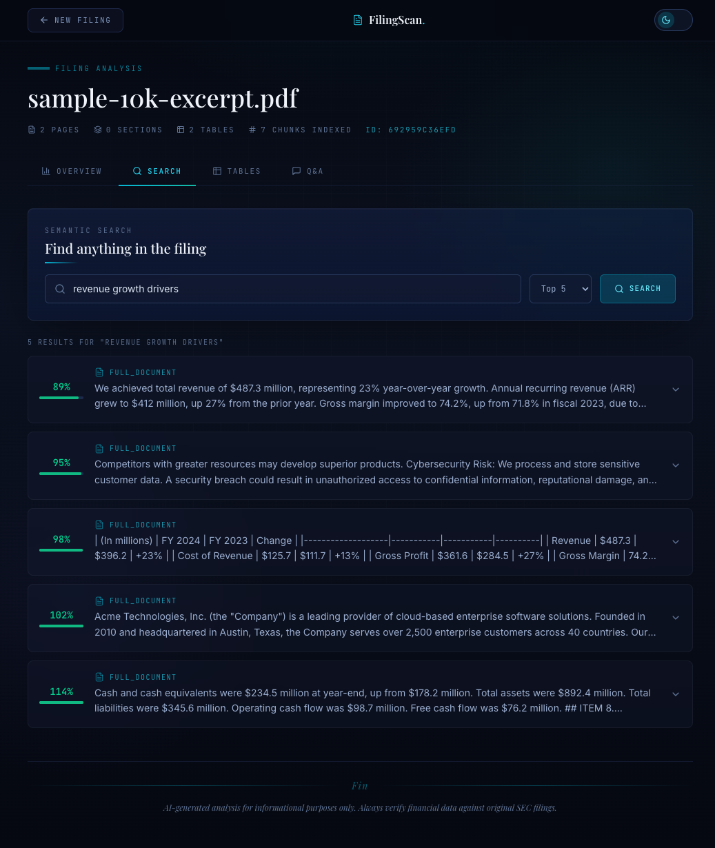
Search#

def search_index(session_id: str, query: str, top_k: int = 5) -> list[dict]:
    """Search a document's index for relevant chunks."""
    db = lancedb.connect(settings.vector_db_path)
    table_name = f"doc_{session_id}"

    if table_name not in db.table_names():
        raise ValueError(
            f"No index found for session {session_id}. Upload a document first."
        )

    table = db.open_table(table_name)
    query_vector = embed_texts([query])[0]

    results = (
        table.search(query_vector)
        .select(["text", "section", "chunk_index", "token_count", "doc_filename"])
        .limit(top_k)
        .to_pandas()
    )

    return [
        {
            "text": row["text"],
            "section": row["section"],
            "chunk_index": int(row["chunk_index"]),
            "score": float(row.get("_distance", 0.0)),
            "doc_filename": row["doc_filename"],
        }
        for _, row in results.iterrows()
    ]

The search path is: embed the query with the same BGE-M3 model, run a nearest-neighbor search on the session's table, return the top-k results with their text, section label, and distance score. LanceDB returns _distance (L2 distance by default on normalized vectors, which is monotonically related to cosine similarity). Lower is better.

Each result carries its section field. When the LLM receives search results for "What are the key risk factors?", it also sees that chunks came from the "Risk Factors" section — not from the executive summary or the auditor's note. This section metadata is what makes answers citable and trustworthy.

Putting It All Together: The Upload Pipeline#

When a user uploads a document, the full pipeline runs in sequence:

Parse: Extract text and sections from the PDF (covered in Blog 2).
Chunk: chunk_document_sections() splits each section semantically, falling back to full-text chunking if needed.
Index: create_index() embeds all chunks with BGE-M3 and writes them to a LanceDB table.
Ready: The session is searchable. Subsequent MCP tool calls (search_document, ask_question) hit this index.

For a 40-page SEC filing, the numbers look like this:

Stage	Time	Output
PDF parsing	~1.2s	15 sections, ~18,000 words
Semantic chunking	~0.8s	72 chunks (avg 245 tokens each)
BGE-M3 embedding	~2.1s	72 vectors, 1024 dims each
LanceDB write	~0.1s	1 table, ~295KB
Total	~4.2s	Searchable index

Under five seconds from PDF upload to a fully searchable vector index. No external services. No API calls for embedding. Everything runs locally.

Naive vs. Semantic: A Concrete Comparison#

To make the difference tangible, I ran both approaches on the same 10-K and searched for "What drove revenue growth in the cloud segment?"

Naive chunking (512-token fixed window):

Top result: "...increased 12% year-over-year. The following table summarizes..." (cuts off before mentioning cloud)
Second result: "...cloud services segment contributed $1.8 billion in annual recurring..." (no growth context)
The answer requires synthesizing across chunks that weren't designed to be related.

Semantic chunking (same 512-token budget):

Top result: "Total revenue for the fiscal year was $4.2 billion, a 12% increase. Growth was primarily driven by the cloud services segment, which saw 28% year-over-year subscription revenue growth. The company expects continued momentum through 2026." (complete thought)
The answer is in the chunk. No synthesis required.

The semantic chunker kept the revenue figure, the growth attribution, and the forward-looking statement together because those sentences have high cosine similarity — they discuss the same topic. The naive chunker split them because they happened to fall across a token boundary.

Configuration Reference#

All chunking and embedding parameters live in a single Pydantic config:

from pydantic import BaseModel, Field

class Settings(BaseModel):
    # Embedding model
    embedding_model: str = "BAAI/bge-m3"
    embedding_dim: int = 1024

    # Chunking
    chunk_size: int = 512
    similarity_threshold: float = 0.5
    min_sentences: int = 2

    # LanceDB
    vector_db_path: str = "data/vectors"

    # Search
    top_k: int = 5

Tuning guidance:

Shorter documents (< 10 pages): Consider chunk_size=256 for more granular retrieval.
Highly structured documents (contracts, regulations): Lower similarity_threshold to 0.4 — transitions between clauses are subtler than between 10-K sections.
Long narrative documents (earnings transcripts): Raise top_k to 8 — relevant context is often spread across more passages.

What's Next#

The vector index is the retrieval backbone. But raw search results are not answers. In the next post, I'll cover the AI layer that sits on top: how Bedrock Claude Haiku generates summaries from the full document, how Claude Sonnet answers questions grounded in search results, and the prompt engineering patterns that keep the model from hallucinating beyond what the document actually says.

Next up: Blog 4 — AI Summarization & Q&A with Bedrock Claude.